20150516

Final Project: Best Vacation Cities in Door County, WI

Goal and Background:

This project was created to determine what the best vacation cities in Door County. Specifically, the objective was to find cities close to major roads for ease of access, close to parks, and near popular recreation attractions. This would be useful information for tourists and travel agencies in helping determine possible destinations or places to stay in Door County.    
 
Methods:

All data was first put into the same projection. Following this, Door County was selected and made into a new feature layer out of Wisconsin county data. This new Door County feature class was then intersected with U.S. recreation spots, parks, major roads, and city data to obtain feature classes that contain data for only that county. The Door County cities feature class was then buffered for a two-mile radius and intersected with the Door County roads feature class to obtain a feature class that contains cities within two miles of a major road. The Door County Parks feature class was dissolved to remove any boundaries within that featured class. The parks were then buffered and intersected with the Road cities feature class to find cities within two miles of a park. The Door County Recreation feature class was then buffered for a two mile radius and intersected with the new Park Cities feature class to obtain a feature class contain the best vacation cities.   

 
Figure 1. Date flow model to obtain Door County vacation cities.    

Results:
Figure 2. Results of geoprocessing data for Door County to determine cities closest to major roads, parks, and recreation facilities.


Sources:  

ArcGIS Content Team. (2003, 12 12). U.S. Major Highways. Data & Maps for ArcGIS . ESRI.
ArcGIS Content Team. (2005, 3 20). U.S. National Atlas Citites. Data & Maps for ArcGIS . ESRI.
ArcGIS Content Team. (2013, 4 26). U.S. Parks. Data & Maps for ArcGIS . ESRI.
ArcGIS Content Team. (2013, 4 18). U.S. Recreation Areas . Data & Maps for ArcGIS . ESRI.
Jarosh, J. (2013). Retrieved May 14, 2015, from Door County Visitor Bureau: www.DoorCounty.com/media
Jarosh, J. (2015). Tourism Spending Up $10 Million in Door County Last Year. Retrieved May 14, 2015, from Door County Wisconsin: http://doorcounty.com/2014/05/02/tourism-spending-up-10-million-in-door-county-last-year
Price, M. (2014). Mastering ArcGIS, Sixth Edition. McGraw Hill.

20150507

Vector Geoprocessing

Goal and Background:
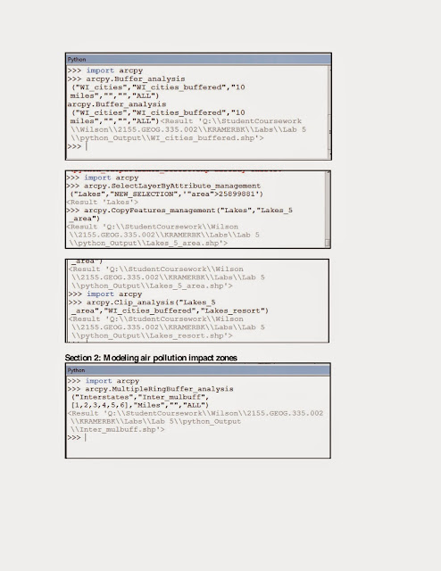
The goal of this exercise was to show my ability to properly choose and apply geoprocessing tools to determine the suitable habitat for bears in the study area of Marquette County, Michigan as well as my ability to use geoprocessing tools through basic scripting in python.
 
Methods:
Part 1: Bear Habitat Suitability Modeling
First I created a feature class from the XY table of the bear data that was in an excel document. Next I added all the necessary data files to ArcMap and used the Intersect tool to create a new feature class that contains the ID number of the bears and the land cover type from the feature classes that contain the bear locations and the land cover. I then selected the top three habitats with the most bears. 
Next I determined what habitat was suitable for the bears by creating a new feature class that contained only the top three bear habitats. I then used the buffer tool (with the dissolve function) to select habitat within 500 meters of a stream. I intersected these two buffered layers and the result was the suitable bear habitat. 
I then determined what of the suitable bear habitat was located on Department of Natural Resources (DNR) land. I used the Dissolve tool to remove the different units on the DNR managed land feature class. I then used to intersect tool on the DNR feature class and the suitable bear habitat feature class to create a feature class containing suitable bear habitat on DNR land. 
 
Part 2: Introduction to Python Scripting


Results:
 Figure 1. This map demonstrates the results from section 1 as well as my data flow model for finding the most suitable habitat for bears in the study area.  

 Figure 2. This map demonstrates the results from section 1 of the python scripting showing the suitable areas for the development of tourist resorts. 

 Figure 3. This map demonstrates the results from section 2 of the python scripting showing the air pollution impact zones around the interstates in Wisconsin. 

Sources:  
Part 1: Michigan Department of Natural Resources (DNR) and Environmental Systems Research Institute (Esri).  
Part 2: Price, Maribeth. 2014. Mastering ArcGIS. 6th Edition CD. McGraw Hill. Lake data from Wilson, Cyril 2012, A comprehensive Lake features for Wisconsin, Unpublished data. 

20150403

Multiple Criteria Query

Goal and Background:
The goal of this exercise was to showcase my skills in composing and implementing query expressions to extract data components from a database.
Methods:
Part 1:
Using U.S. county data, I wrote a multiple criteria query that returned counties with population between 3000 and 4000 people in 2010 and also all counties in 2010 that had a population density of at least 1000 persons per square mile. In the end it looked as follows:

POP2010 >= 3000 AND POP2010 <= 4000 OR POP10_SQMI >= 1000


Next I wrote a multiple criteria query that returned records for counties in Wisconsin, Texas, New York, Minnesota, and California where male population is greater than female population and also for these states the number of seniors (age 65 and above) is over 6500. In the end it looked as follows:

STATE_NAME IN ( 'Wisconsin', 'Texas', 'New York', 'Minnesota', 'California') AND MALES > FEMALES AND AGE_65_UP >6500
I then modified that query  to add all other seniors in Washington, Maryland, Illinois, Nebraska, District of Columbia and Michigan who reside in counties that have more than 30,000 housing units to the result obtained in query 2. In the end it looked as follows:

STATE_NAME IN ( 'Wisconsin','Texas', 'New York', 'Minnesota', 'California') AND MALES > FEMALES AND AGE_65_UP >6500 OR STATE_NAME IN ( 'Washington', 'Maryland', 'Illinois', 'Nebraska', 'District of Columbia', 'Michigan') AND AGE_65_UP >0 AND HSE_UNITS >30000
Part 2:
Using Wisconsin data, I developed a query that returned cities in Wisconsin, in 2007, with a population between 15,000 and 20,000 people, area of the city is at least 5 square miles in land area, and also female population is greater than males, and also the cities are within 2 miles of a lake. In the end it looked as follows:
 ( "POP2007" >=15000 AND "POP2007" <=20000) AND "AREALAND" >=5 AND "FEMALES" > "MALES"
I also developed a multiple criteria query to calculate the total length of the following rivers in Wisconsin: CHIPPEWA R, EAU CLAIRE R, 'EMBARRASS R, FISHER R, HUNTING R, KINNICKINNIC R, MAUNESHA R, MILWAUKEE R, MOOSE R, NAMEKAGON R, PELICAN R, PLATTE R, and POTATO R. In the end it looked as follows:

"PNAME" IN ('CHIPPEWA R', 'EAU CLAIRE R', 'EMBARRASS R', 'FISHER R', 'HUNTING R', 'KINNICKINNIC R', 'MAUNESHA R', 'MILWAUKEE R', 'MOOSE R', 'NAMEKAGON R', 'PELICAN R', 'PLATTE R', 'POTATO R')

Results:

Figure 1. This map demonstrates the results of my first query, determining counties with population between 3000 and 4000 people in 2010 and also all counties in 2010 that had a population density of at least 1000 persons per square mile.


Figure 2. This map demonstrates the results of my second query, demonstrating counties in Wisconsin, Texas, New York, Minnesota, and California where male population is greater than female population and also for these states the number of seniors (age 65 and above) is over 6500.

Figure 3. This map demonstrates the results of my third query, demonstrating modifications to the second query to include all other seniors in Washington, Maryland, Illinois, Nebraska, District of Columbia and Michigan who reside in counties that have more than 30,000 housing units. 
Figure 4. This map demonstrates the results of my fourth query, demonstrating cities in Wisconsin, in 2007, with a population between 15,000 and 20,000 people, area of the city is at least 5 square miles in land area, and also female population is greater than males, and also the cities are within 2 miles of a lake. 


Figure 5. This map demonstrates the results of my fifth query, demonstrating the following rivers in Wisconsin: CHIPPEWA R, EAU CLAIRE R, 'EMBARRASS R, FISHER R, HUNTING R, KINNICKINNIC R, MAUNESHA R, MILWAUKEE R, MOOSE R, NAMEKAGON R, PELICAN R, PLATTE R, and POTATO R used to calculate their total length. 
Sources: Wisconsin data was given to us by Dr. Wilson. All USA data was from Mastering ArcGIS by Maribeth Price.  

20150316

Downloading and Mapping GIS Data

Goal and Background:
The main goal of this lab was to learn how to transform a stand-alone table that contained relevant data into an attribute table so that the data can be mapped. Another goal of the lab was to become familiar with the U.S. Census Bureau’s website so that it is easy to find data and information that can be used in GIS.  

Methods:
Step 1: I visited the American Factfinder website of the U.S. Census Bureau
Step 2: I downloaded and unzipped the census attribute table for the counties of the state of Wisconsin.
Step 3: I viewed both the meta data and the tabular data in MS Excel and changed the number data in Excel from “general” to “number.”
Step 4: I saved the CSV file as an MS Excel file.
Step 5: I added the MS Excel file to ArcMap and reviewed the attribute table to make sure it was transferred correctly.
Step 6: I downloaded and unzipped the shapefile for the counties of the state of Wisconsin.
Step 7: I added the WI shapefile to ArcMap.
Step 8: I joined the WI shapefile and the population data table together through a join based on their GEO ID.
Step 9: I changed the symbology of the shape file to display a graduated color scheme that coincided with the population of the Wisconsin counties normalized for area.
Step 10: I repeated steps 1-5 and steps 7-9 using number of Housing units instead of county population.
Step 11: I built an appealing layout for both maps and changed the projection of the data frame to a State Plane projection for Central Wisconsin. 

Results: 

 Figure 1. This map represents the population of Wisconsin counties normalized for county area demonstrated by a color gradient. This map was created using data downloaded from the U.S. Census Bureau website which was then transformed into an MS Excel file and joined with a table so that the information could be mapped.
 Figure 2. This map represents the number of housing units of Wisconsin counties demonstrated by a color gradient. This map was created using data downloaded from the U.S. Census Bureau website which was then transformed into an MS Excel file and joined with a table so that the information could be mapped.

Sources: United States Census Bereau (2010). American Factfinder. Retrieved from http:// http://factfinder.census.gov/faces/nav/jsf/pages/searchresults.xhtml?refresh+t.

20150224

Coordinate Systems and Map Projections


Goal and Background:
This project aims to show that I know the difference between geographic projected coordinate systems and that I am able to apply this knowledge to GIS data that has had some or all of this information removed from it. Furthermore this project aims to show that I am able to identify projection error in GIS data and project or reproject the data appropriately so that it might be usable in GIS.

Methods:
Part 1: Creating the World Projections
Section 1:
To create the first projection of the world map I added shapefiles containing the global countries and a grid. I then set the coordinate system of the data frame to WGS 1984.

Section 2:
I then added data frames and placed the same shapefiles within them. In the end I had five data frames with the coordinate systems: WGS 1984, Mercator Projection, Sinusoidal projection, Equidistant-Conic projection, and Robinson projection.

Part 2: Creating the Wisconsin and United States Projections
Section 1:
To make the projection of the Wisconsin map seen in Figure 1, I insert a new data frame and added a shapefile that contained the states of the United States. I then selected Wisconsin and made a layer from that selection and saved it as its own shapefile. I then changed the projection of this shapefile to UTM, NAD 1983, Zone 16N.

Section 2:
To make the projection of the United States found in Figure 1, I created a new data frame and added a shapefile containing the states and a shapefile containing state roads. I changed the projection of the roads shapefile to match that of the states shapefile. I then used the Project tool in Arc Toolbox setting the input to the roads shapefile and imported the states shapefile to be the output. Finally, I changed the projection of the data frame to North American Lambert Conic.

Part 3: Creating the Projection of Wisconsin Counties and Rivers
First, I added the shapefile that contain the central Wisconsin counties. This shapefile did not have a projection or coordinate system. Based on the metadata provided, I gave it the geographic coordinate system GCS North American 1983 and the projection of North America Equidistant Conic. I then added a shapefile containing the rivers in those counties. This shapefile had a different projection than that of the county shapefile. I used the project tool to match the rivers shapefile projection to that of the counties.

 
Results:


Figure 1. The first five maps display the world shown in different projection possibilities which were changed through the properties window of the data frame. The bottom left map displays a Wisconsin shape file made from a selection from an United States map with the projection changed to a Transverse Mercator projection again using the data frame properties window. The bottom right map displays a map with cohesive projections created from data with different projections originally. The changes were made using the Project tool in the ArcToolbox. 


Figure 2. This map displays the rivers and counties of central Wisconsin produced from data that originally did not have projections or projections that match. The shapefile was first given a coordinate system and projection based on the metadata and the rivers shapefile was then added. This shapfile's projection was then changed using the ArcToolbox to match the county shapefile.  


Sources: Mastering ArcGIS by Maribeth Price.